Regression Modelling with SurPyval
This section is about how we can understand the effect that covariates can have on survival times. As per the other entries in these docs, let’s import some useful packages, as such, for the rest of this page we will assume the following imports have occurred:
import surpyval as surv
import numpy as np
from matplotlib import pyplot as plt
Regression survival modelling with surpyval is very easy. This page will take you through a series of scenarios that can show you how to use the features of surpyval to get you the answers you need.
Semi-Parametric - Cox Proportional Hazards Model
The first example is the Cox Proportional Hazards model. In this example we will use the data from Krivtsov et al. This data set is the results of testing tires time to failure with measurements about those tires. The authors of this paper intended to determine what factors affected tire reliability.
from surpyval.datasets import Tires
from surpyval import CoxPH

x = Tires.data['Survival']
c = Tires.data['Censoring']
Z = Tires.data[['Tire age', 'Wedge gauge', 'Interbelt gauge', 'EB2B', 'Peel force',
    'Carbon black (%)', 'Wedge gauge×peel force']]
model = CoxPH.fit(x=x, Z=Z, c=c)
model
Regression SurPyval Model
=========================
Type                : Proportional Hazards
Kind                : Cox
Parameterization    : Semi-Parametric
Parameters          :
    beta_0  :  2.109496593744941
    beta_1  :  -9.686078593632743
    beta_2  :  -10.67809536747068
    beta_3  :  -13.67594841333851
    beta_4  :  -34.29448581473381
    beta_5  :  -48.35286747450483
    beta_6  :  20.84037862912251
We can see that we have a micture of coefficients. We can check the p-values:
print(model.p_values)
[0.13000628, 0.03677433, 0.02074066, 0.0918419 , 0.01200102, 0.14831534, 0.01867559]
We can asee that it is only 1, 2, 4, and 6 that are significant at the 0.05 level.
We can redo the model using only those covariates:
from surpyval.datasets import Tires
from surpyval import CoxPH

x = Tires.data['Survival']
c = Tires.data['Censoring']
Z = Tires.data[['Wedge gauge', 'Interbelt gauge', 'Peel force', 'Wedge gauge×peel force']]
model = CoxPH.fit(x=x, Z=Z, c=c)
print(model.p_values)
model
[0.02207978 0.01368372 0.00956108 0.01030372]

Regression SurPyval Model
=========================
Type                : Proportional Hazards
Kind                : Cox
Parameterization    : Semi-Parametric
Parameters          :
    beta_0  :  -9.313960179920473
    beta_1  :  -7.069295556681021
    beta_2  :  -27.413473066027667
    beta_3  :  18.105822313415462
All the coefficients can now be seen to be significant. It also shows that as the wedge gauge, interbelt gauge, and peel force increase, the hazard rate will decrease and the life will therefore increase. The opposite is the case for the wedge gague x peel force coefficient.
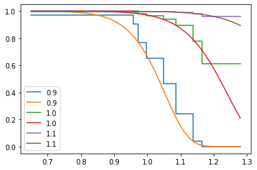
We can plot the survival curves of the average tire and the 10% above and 10% below average tire:
Z_mean = Tires.data[['Wedge gauge', 'Interbelt gauge', 'Peel force', 'Wedge gauge×peel force']].mean().values

plot_x = np.linspace(x.min(), x.max())
for f in [0.9, 1., 1.1]:
    plt.step(plot_x, model.sf(plot_x, Z=Z_mean * f), label=f)
plt.legend()
We can see that as the covariates increase there is a decrease in the probability of survival up to 1.2. The Semi-Parametric nature of the model can also be seen clearly in this plot. You can see that the baseline is non-parametric, but the baseline has been affected by the covariates.
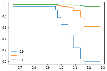
Parametric Proportional Hazards Modelling
In the above example we used a semi-parametric model where the ‘baseline’ hazard rate was a non-parametric model but the hazard was multiplied by a parametric function of the covariates. We can use fully parametric models instead. These come with the advantages of parametric models, namely extrapolation, but are also disadvantaged by the assumption needed about the shape of the distribution. SurPyval has two Proportional Hazard models that are ready to use with any number of covariate inputs (just like the CoxPH model); these are the ExponentialPH and the WeibullPH models. We will analyse the tires data using the Weibull Proportional hazards model.
from surpyval.datasets import Tires
from surpyval.regression import WeibullPH

x = Tires.data['Survival']
c = Tires.data['Censoring']
Z = Tires.data[['Wedge gauge', 'Interbelt gauge', 'Peel force', 'Wedge gauge×peel force']]
weibull_ph_model = WeibullPH.fit(x=x, Z=Z, c=c)
weibull_ph_model
Parametric Regression SurPyval Model
====================================
Kind                : Proportional Hazard
Distribution        : Weibull
Regression Model    : Log Linear (Exponential)
Fitted by           : MLE
Distribution        :
    alpha: 0.24255057163126237
    beta: 16.057788534593193
Regression Model    :
    beta_0: -9.165054735694651
    beta_1: -7.998600691841399
    beta_2: -27.50328118957879
    beta_3: 18.38550168401127
You can see from the above that the coefficients for the covariates are very similar.